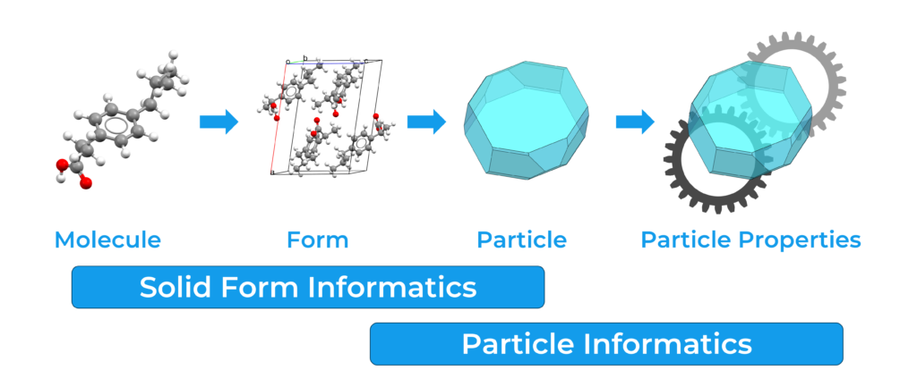
How to Visualize and Analyse Surfaces Using Mercury
The arrangement of molecules within a crystal structure affects the shape of the particles, and hence the way they behave in the stages of formulation and manufacturing.
The particle informatics tools included in the CSD-Particle suite help analyse structural features to understand how these can impact the mechanical properties of the particles, and rationalize the surface chemistry and topology of crystal facets.
In this blog, you will learn how to use the desktop molecular visualizer software Mercury to:
- Identify and analyse potential slip planes
- Perform surface analysis
- Calculate Full Interaction Maps on surfaces
Follow the link to read a use case where some of the tools included in the CSD-Particle suite were used to study the crystal morphology of cipamfylline.
The Slip Planes Component
The presence of slip planes in a crystal structure of a pharmaceutical material is particularly crucial as it influences how the particle compacts and bends, which impacts tabletting.
For our analysis, we will use the crystal structure of acetylsalicylic acid, also known as aspirin, CSD Entry ACSALA01. To run the “Slip Planes” component:
- Open Mercury and search for ACSALA01 on the “Structure Navigator” bar;
- Go to “CSD-Particle” > “Slip Planes” > “Calculate”.
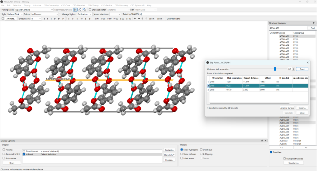
When the slip planes calculation is completed, the results appear on a table (Figure 1, see also Figure 3) which includes:
- Orientation: the Miller plane that sits parallel to the slip plane;
- Slab separation: the shortest distance between the slabs of molecules on either side of the slip plane (Å); note that a negative value indicates an overlap of the two slabs of molecules;
- Repeat distance: the perpendicular distance to the next equivalent slip plane (Å);
- Offset: the perpendicular distance from the slip plane to the parallel Miller plane (Å);
- H-bonded: whether or not intermolecular hydrogen bonds cross the slip plane;
- Perpendicular planes: a list of slip planes with orientations perpendicular to the selected one.
By clicking on the plane of interest listed on the table, you can easily visualize it within the crystal packing on the main window of Mercury. This will bring up the “Packing and Slicing” window where you can customize several visualization features, including how the plane is displayed and modify parameters like the depth and area of the plane (Figure 2).
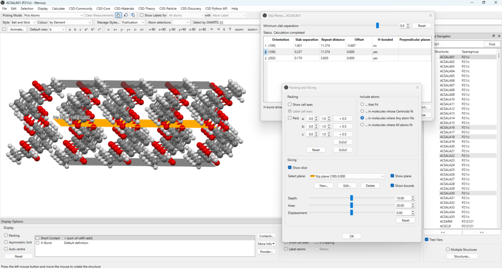
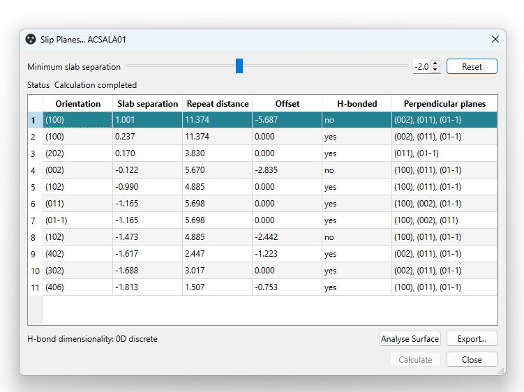
Additionally, the minimum slab separation can be modified and decreased to display more planes (Figure 3, top), enabling users to investigate and visualize a variety of potential slip planes directly on the structure of interest.
As it can be seen in Figure 3, in CSD Entry ACSALA01 there are two slip planes parallel to the (100) Miller plane, one of which is crossed by hydrogen bonds. These can be easily visualized by selecting “H-bond” from the “Display Options” tab at the bottom left of the Mercury window (Figure 4).
Some of the conclusions that can be extracted from this analysis are:
- The presence of several slip planes in aspirin, many of which are interconnected to one another, matches the experimental observations on its mechanical properties, which determined that the crystal structure of aspirin is quite brittle and easy to break apart [1], [2];
- This is also supported by the fact that some of the slip planes are not connected by hydrogen bonds, which makes it easier for the planes to slip when under compression and disrupt the crystal structure;
- Among the slip planes that are instead crossed by hydrogen bonds, the one that is parallel to the (100) Miller plane connects two carboxylic acids of consecutive aspirin molecules;
- From the hydrogen bond dimensionality of the latter (which can be found at the bottom left of the “Slip Planes” panel), it can be observed that these dimers are discrete and do not develop in chains, sheets, or networks.
If you are interested in analysing these features for other slip planes in the structure, this can be easily done in Mercury by selecting the plane of interest in the “Slip Planes” panel.
The Surface Analysis Component
The visualization of surfaces and the analysis of features that characterize them, such as the presence of hydrogen bond donors/acceptors, the surface roughness, and the surface charge, enable an in-depth understanding of the surface topology and surface chemistry of a particle.
The component to perform this analysis in Mercury is called Surface Analysis. To run this component:
- Go to “CSD-Particle” > “Surface Analysis”, or
- Go to “Analyse Surface” from the “Slip Planes” panel shown in detail in Figure 3; note that in this case the surface analysis will be performed on the plane that is selected on the “Slip Planes” panel and using the corresponding calculated parameters.
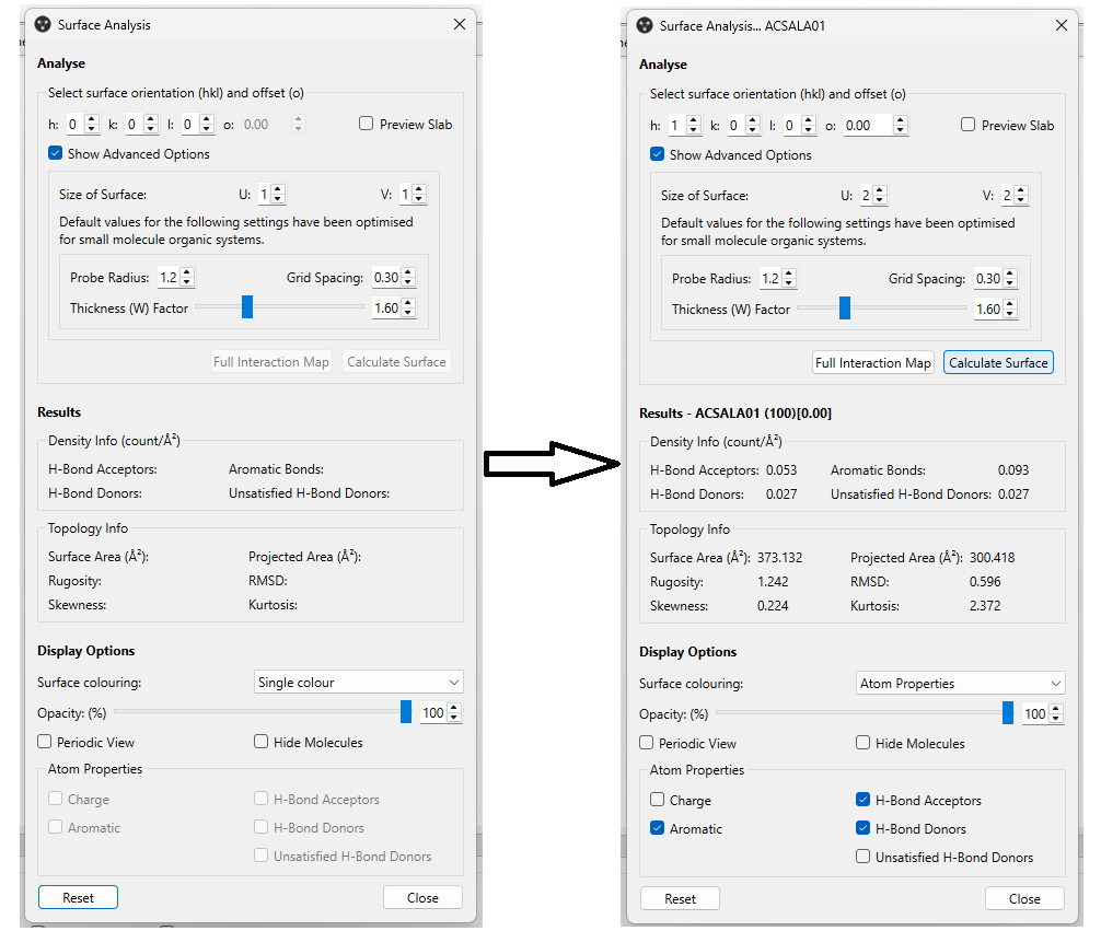
The “Surface Analysis” panel (Figure 5, left) will open. This is divided into three areas:
- Analyse: here you can select the surface orientation that you are interested in by specifying its h, k, and l indices; you can also set a surface offset value, useful to modify the surface termination, and preview the slab for the set offset directly on the visualization panel of Mercury; additionally, you can modify advanced options, including the size of the surface, and the probe radius and grid spacing used to calculate the surface;
- Results: here you can see the results from the surface calculation, including the density of H-bond acceptors, donors, aromatic bonds, and unsatisfied H-bond donors (count/Å2); additionally, you can see topology information, such as the surface area (Å2) and the rugosity; you can find out more about each of these details by hovering over them with your mouse cursor;
- Display Options: the final section enables you to select and modify the features that you want to visualize, including the surface colouring, its opacity, and some atom properties that you might be interested in.
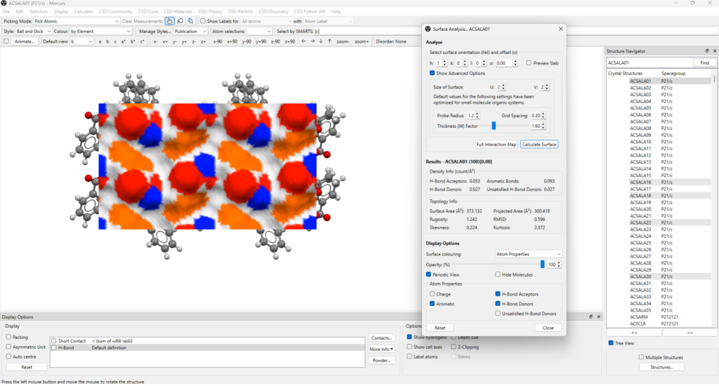
By selecting the settings reported in Figure 5 on the right, and then clicking on “Calculate Surface”, you’ll be able to visualize the calculated surface on the visualization panel of Mercury.
This is the (100) surface with 0.00 offset, corresponding to the plane that includes the hydrogen bonds from the discrete dimers that was highlighted in the section above.
Reported in Figure 6 are the results from this calculation: areas of the surface which are H-bond donors (blue), H-bond acceptors (red) and aromatic interactions (orange).
The “Surface Analysis” panel also shows the values of surface density for these interactions, and the surface area value.
Some of the conclusions that can be extracted from this analysis are:
- The presence of numerous hydrogen bond donors, acceptors, and aromatic groups on the (100) surface with 0.00 offset suggests that more aspirin molecules could easily pack along the direction perpendicular to this surface and satisfy some of the unsatisfied donors detected (see the details in Figure 5, right);
- This can indeed occur quite easily, but the same can’t be said for the consecutive parallel surface, the (100) surface with -5.69 offset (the one with no hydrogen bonds across); in fact, this surface appears to have no H-bond donors, indicating that the crystal growth along this direction is more likely to be very slow or to terminate with this surface.
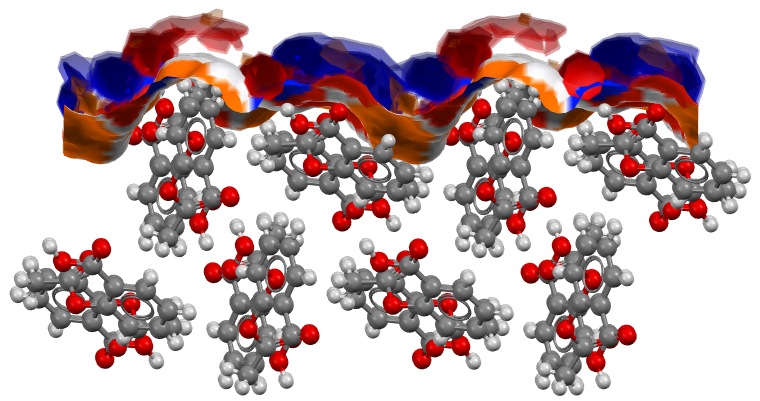
Full Interaction Maps on Surfaces
As part of the Surface Analysis component, Full Interaction Maps on Surfaces (FIMoS) can also be calculated to further explore the surface chemistry of a particle.
Here you can find more information on how FIMoS are obtained. For the purpose of this blog, we will only highlight that FIMoS enable users to quickly visualize the preferred positions for interactions on a crystal surface.
To run this calculation:
- Select the (011) plane from the “Slip Planes” panel > “Analyse Surface”;
- Click on “Full Interaction Map” on the “Surface Analysis” panel > “Calculate Surface Maps”; note that a variety of settings can be changed in the “Full Interaction Maps on Surface” panel.
The results are then shown on the main visualization window of Mercury, as it can be seen in Figure 7.
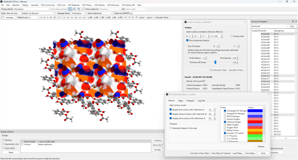
The choice of the (011) plane for this analysis comes from experimental observations: the crystals of aspirin seem to prefer a needle-like morphology, with crystals growing faster along the b-axis direction, where {011} planes are the capping surfaces.
From the FIMoS calculation on this surface, it can be easily identified the reason behind this preference:
- Firstly, this surface is rich of regions where it is likely for hydrogen bond donor and acceptor groups to sit, as well as for aromatic interactions to take place;
- Secondly, the addition of another layer of aspirin molecules along the direction perpendicular to the (011) surface would form another equivalent surface that is hence rich of regions where the same stabilizing interactions are expected to form (Figure 8);
- For this reason, this is likely to be the preferential direction of growth for crystals of aspirin.
Next Steps
Find out more about the CSD-Particle tools in the following publications:
- Predicting mechanical properties of crystalline materials through topological analysis, CrystEngComm, 2018, 20, 2698-2704.
- Surface Analysis─From Crystal Structures to Particle Properties, Cryst. Growth Des. 2024, 24, 10, 4160–4169.
To discuss further and/or request a demo with one of our scientists, please contact us via this form or .